Tissue & Artifacts Detection

HistoKit provides tissue detection and artifact identification on whole-slide images (WSI). These artifacts may negatively impact both the computational cost and the quality of results produced by downstream image analysis algorithms. Below is a brief description of the methods currently used.

Algorithms description

Tissue detection

Artifact detection

Run tissue and artifacts detection

The script run_tissue_seg.py is used to execute the tissue segmentation and artifact detection algorithms. Below is a description of the parameters accepted by the script, along with explanations of their functionality.

Configuration

Common settings

Parameter	Type	Default	Description
--wsi_dir	str	/Data/	Input directory containing WSIs.
--out_dir	str	/Results/	Directory where results will be saved.
--vis_mag	int	0.625	Magnification for saved visualizations.
--overwrite	bool	False	If set, existing output files are overwritten.

Tissue detection settings

The tissue detection stage is executed on the CPU. It is possible to increase the number of workers to process multiple .svs files in parallel. However, when doing so, it is important to monitor your system’s RAM usage, particularly when working with large WSI images.

Parameter	Type	Default	Description
--run_tis_det	bool	True	Run tissue/background detection.
--fill_holes	bool	True	Fill holes inside tissue regions.
--close_disk_r	int	2	Radius for disk kernel during morphological closing.
--open_disk_r	int	2	Radius for disk kernel during morphological opening.
--tissdet_mag	float	2.5	Magnification used for tissue detection.
--remove_small_objects	bool	True	Remove small tissue areas (which are potentially too small for further analysis) after tissue segmentation.
--workers	int	4	Number of workers used during tissue detection.

Artifact detection settings

The artifact detection stage using the GrandQC model can be accelerated by leveraging CUDA-enabled GPU processing. This stage makes use of the tissue masks obtained from the thresholding-based detection step. This significantly reduces the computation time, as artifact prediction is performed only on regions that contain tissue.

Parameter	Type	Default	Description
--run_artifacts_det	bool	True	Run artifact detection step.
--save_confidence_maps	bool	True	Save per-class confidence maps.
--device	str	cuda	Device used for inference (cuda/cpu).
--workers_per_slide	int	6	Number of workers used during patch extraction & batching.
--batch_size	int	64	Mini-batch size for inference.
--grandqc_model	str	../HE/models/GrandQC_MPP1.pth	Path to GrandQC checkpoint.
--grandqc_mpp	float	1.0	Micron-per-pixel for the GrandQC model (1.0 corresponds to 10x magnification).
--patch_size_model	int	512	Patch size for model input.
--save_mag	float	2.5	Magnification for saving final segmentation mask.
--encoder_model	str	timm-efficientnet-b0	Encoder architecture for GrandQC backbone.
--encoder_model_weights	str	imagenet	Pretrained weights for encoder initialization.
--overlap	float	0.75	Overlap ratio between extracted patches.
--blending_mode	str	gaussian	Method for merging overlapping patch predictions.
--blending_sigma	float	None	Sigma used for Gaussian blending (ignored for average mode).

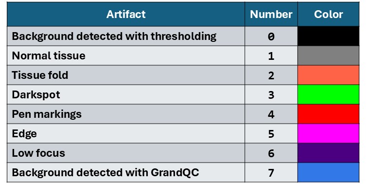
Artifacts Color Mapping

The GrandQC model generates masks with integer values from 0 to 7. During visualization, these values are mapped to corresponding colors. The table below presents the mapping between artifact classes and their visual representations, along with example artifacts marked on the slides. Note that the original model was not trained on some specific tissue types, which may lead to inaccurate artifact segmentation in certain cases.

Output Folders

Folder name	Description
masks/	Masks with detected tissue (two classes: background and tissue), saved as .mat files.
masks_grandqc/	Masks with detected artifacts using the GrandQC model, saved as .mat files.
grandqc_confidence_maps/	Confidence maps for each artifact type detected by the GrandQC model, saved as .mat files.
bg_thr_hist/	Histograms of background thresholds used for tissue detection.
raw_small/	Tissue images before artifact and background detection (images saved at the magnification specified by the --vis_mag parameter).
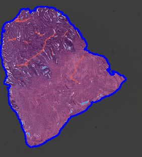
bg_removal_contour_vis/	Background removal visualizations with blue contours (images saved at the magnification specified by the --vis_mag parameter).
grandqc_overlay_vis/	Artifact detection results overlaid on tissue regions (images saved at the magnification specified by the --vis_mag parameter).

Example Results

masks

Folder containing .mat files with masks generated during tissue detection. Each file contains the following fields:

Key	Description
basename	Basename of the corresponding tissue image (filename without the .svs extension).
mask_bg	Binary tissue mask (uint8 2D array). Tissue pixels are labeled as 1 and background pixels as 0. The mask is generated for the entire slide (regions are not separated).
ind_WSI	Indices of WSI pyramid levels (MATLAB-style indexing starting at 1).
ratio	Scaling ratio for each pyramid level, computed as: size of largest WSI layer / size of the given layer.
scale_val	Final scale factor applied to masks. Computed as: mask magnification / magnification of the largest WSI layer.
thr	Threshold values used for tissue detection for the R, G, and B channels.
mask_mag	Magnification at which the mask is stored.
mpp	Microns-per-pixel (MPP) value of the slide. If unavailable in metadata, it is estimated as: 10 / magnification of the largest WSI layer.
mag_l0	Magnification of the largest-resolution WSI layer (highest detail level).

masks_grandqc

Folder containing .mat files with masks after tissue detection. Files have the following structure:

Key	Description
basename	Basename of the tissue file (filename without the .svs extension).
mask_art	List of artifact masks for each detected region. Each element is a uint8 2D array containing values in the range 0–7 corresponding to artifact classes. Each region is stored as a separate mask.
ind_WSI	Indices of WSI pyramid layers (MATLAB-style indexing starting at 1).
ratio	Scaling ratio for each WSI pyramid layer. Computed as: dimension of the largest layer / dimension of the given layer.
scale_val	Scale factor applied to masks, computed as: mask magnification / magnification of the largest WSI layer.
thr	Threshold values used for tissue/background detection for the R, G, and B channels.
bbox	List of bounding box coordinates for each region. Coordinates follow Python indexing (starting at 0).
mask_mag	Magnification at which the masks are stored.
mpp	Microns-per-pixel (MPP) value of the slide. If metadata does not include MPP, it is estimated as: 10/magnification of the largest WSI layer
mag_l0	Magnification of the largest-resolution WSI layer (highest detail level).

grandqc_confidence_maps

Folder containing .mat files with masks after tissue detection. Files have the following structure:

Key	Description
basename	Basename of the tissue file (filename without the .svs extension).
mask_conf	List of confidence score maps for artifact classes for each region. Each element is a uint8 3D array with dimensions (width × height × n_classes). Each slice along the third dimension corresponds to the confidence map for one artifact type. Each region is stored as a separate 3D mask. Confidence scores are scaled to integer values from 0 to 255 and can be displayed as a binary image. For background detected during the thresholding (0 layer) background is white (255 - 100% confidence that pixel belongs to the background) and the tissue area is black (0 - no background).
ind_WSI	Indices of WSI pyramid layers (MATLAB-style indexing starting at 1).
ratio	Scaling ratio for each WSI pyramid level, computed as: dimension of the largest layer / dimension of the given layer.
scale_val	Scale factor applied to the masks, computed as: mask magnification / magnification of the largest WSI layer (``mag_l0``).
thr	Threshold values used for tissue/background detection for the R, G, and B channels.
bbox	List of bounding box coordinates for each region. Coordinates follow Python indexing (starting at 0).
mask_mag	Magnification at which the confidence maps are stored.
mpp	Microns-per-pixel (MPP) value of the slide. If metadata does not include MPP, it is estimated as: 10 / magnification of the largest WSI layer.
mag_l0	Magnification of the highest-resolution WSI layer.

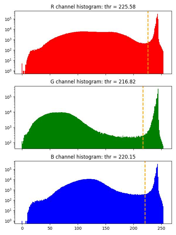
bg_thr_hist

Histograms with background threshold values for each color channel calculated with GaMRed algorithm, or with Otsu method when threshold obtained with GaMRed is too small (smaller than 0.7*255).

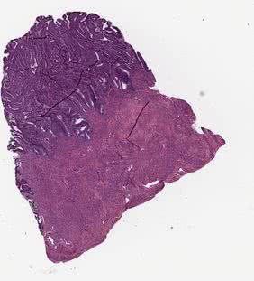
raw_small

Original tissue image saved with the magnification defined by the --vis_mag parameter.

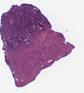
bg_removal_contour_vis

In this folder, the visualizations of tissue detection using the thresholding methods are stored. The contours of detected tissue are drawn on the original image. Image is saved with the magnification defined by the --vis_mag parameter.

grandqc_overlay_vis

In this folder, the visualizations of artifact detection using the GrandQC model are stored. The original image is overlaid with the generated artifact mask, and then the contours of the detected tissue are drawn. Image is saved with the magnification defined by the --vis_mag parameter.

How to Load Regions to Matlab?

Generated artifacts maps are saved to .mat files which can be loaded both with Matlab and Python. The following function can be used to load .mat files generated during artifacts detection step to Matlab.

function [img,mask_all] = load_tiss_masked_histokit(svs_name,mask_name,reg_ID, qual_ind, exclude_art)
% svs_name - name of the svs file
% mask_name - name of the corresponding .mat file
% reg_ID - region ID
% qual_ind - index for wsi layer
% exclude_art - vector of artifacts to exclude:

% BG_THR = 0       # BACKGROUND (after mask detection): black
% NORM = 1         # ART_NORM: gray
% ART_FOLD = 2     # ART_FOLD: orange
% ART_DARKSPOT = 3 # ART_DARKSPOT: green
% ART_PEN = 4      # ART_PEN: red
% ART_EDGE = 5     # ART_EDGE: pink
% ART_FOCUS = 6    # ART_FOCUS: violet
% BG_MODEL = 7     # BACKGROUND (predicted by artifact detection model): blue

% load info about mask
load(mask_name,'mask_art','ratio','bbox',...
    'ind_WSI','scale_val')

% calculate scaling value for selected image resolution mask
scale_val = scale_val*ratio(ind_WSI == qual_ind);

% get bounding box for the region and resize
Box = (bbox(reg_ID,:)+1) / scale_val;

% get location of the region and load image
rows = [Box(1), Box(3)];
cols = [Box(2), Box(4)];

region = {rows,cols};
img = imread(svs_name,'Index',qual_ind,'PixelRegion',region);
figure;image(img)

% get mask of region, resize and apply to image
mask_all = uint8(imresize(mask_art{reg_ID},[size(img,1),size(img,2)]));

% variants we want to exclude are set to 0
mask_all(ismember(mask_all, exclude_art))=0;
mask_all(~ismember(mask_all, exclude_art))=1;

for b=1:size(img,3)
    tmp = img(:,:,b).*mask_all;
    tmp(mask_all == 0) = 255;
    img(:,:,b) = tmp;
end
clear tmp
figure;image(img)

end

Example usage:

% search for original .svs file
svs_name = "224-20_he.svs";
mask_name = "224-20_he.mat";

% check how many regions are there
load(mask_name, "bbox")
load(mask_name, "ind_WSI")
n3 = size(bbox,1);

%iterate over regions
for b=1:n3

    % load region with 10x magnification, that is why are using ind_WSI(2) for our WSI
    exclude_art = [0, 2, 3, 4, 5, 6, 7];
    img = load_tiss_masked_histokit(svs_name,mask_name,b,ind_WSI(2), exclude_art);
    imshow(img);
end

References

• Z. Weng, A. Seper, A. Pryalukhin, et al. GrandQC: A comprehensive solution to quality control problem in digital pathology. Nature Communications 15, 10685 (2024). DOI | GitHub

• M. Marczyk, A. Wrobel, J. Merta, and J. Polanska (2025). Post-Processing of Thresholding or Deep Learning Methods for Enhanced Tissue Segmentation of Whole-Slide Histopathological Images. In: Proceedings of the 18th International Joint Conference on Biomedical Engineering Systems and Technologies – Volume 1: BIOIMAGING. SciTePress, pp. 229–238. ISBN 978-989-758-731-3. DOI | GitHub